Statistical analysis

ParaView Statistics Plugin

The ParaView trunk and the upcoming 3.6.2 release include a statistics plugin. This plugin provides a way to use vtkStatisticsAlgorithm subclasses from within ParaView.

Once the plugin is loaded you should see a new submenu in the Filters menu bar named Statistics that contains

• Contingency Statistics
• Descriptive Statistics
• K-Means
• Multicorrelative Statistics
• Principal Component Analysis

In the near future, there will also be a bivariate correlative statistics filter that provides more summary information than the multicorrelative version.

Using the plugin

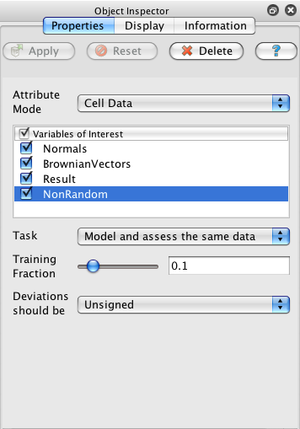
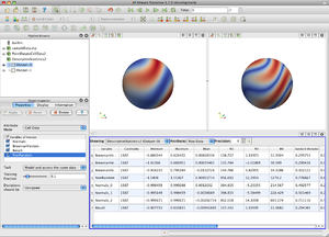
In the simplest use case, just select a dataset in ParaView's pipeline browser, create a statistics filter from the Filter→Statistics menu, hit return to accept the default empty second filter input, select the arrays you are interested in, and click Apply.

Descriptive statistics filter setup.

The default task for all of the filters (labeled "Model and assess the same data") is to use a small, random portion of your dataset to create a statistical model and then use that model to evaluate all of the data. There are 4 different tasks that filters can perform:

1. "Statistics of all the data," which creates an output table (or tables) summarizing the entire input dataset;
2. "Model a subset of the data," which creates an output table (or tables) summarizing a randomly-chosen subset of the input dataset;
3. "Assess the data with a model," which adds attributes to the first input dataset using a model provided on the second input port; and
4. "Model and assess the same data," which is really just the 2 operations above applied to the same input dataset. The model is first trained using a fraction of the input data and then the entire dataset is assessed using that model.

When the task includes creating a model (i.e., tasks 2, and 4), you may adjust the fraction of the input dataset used for training. You should avoid using a large fraction of the input data for training as you will then not be able to detect overfitting. The Training fraction setting will be ignored for tasks 1 and 3.

The first output of statistics filters is always the model table(s). The model may be newly-created (tasks 1, 2, or 4) or a copy of the input model (task 3). The second output will either be empty (tasks 1 and 2) or a copy of the input dataset with additional attribute arrays (tasks 3 and 4).

Caveats

Warning: When computing statistics on point arrays and running pvserver with data distributed across more than a single process, the statistics will be skewed because points stored on both processes (due to cells that neighbor each other on different processes) will be counted once for each process they appear in. We are working to resolve this issue but without forcing a redistribution of the data, it is not simple.

Filter-specific options

Contingency Statistics

This filter computes contingency tables between pairs of attributes (a process known as marginalization). This result is a tabular bivariate probability distribution which serves as a Bayesian-style prior model. Data is assessed by computing

• the probability of observing both variables simultaneously;
• the probability of each variable conditioned on the other (the two values need not be identical); and
• the pointwise mutual information (PMI).

Finally, the summary statistics include the information entropy of the observations.

Descriptive Statistics

This filter computes the min, max, mean, raw moments M2—M4, standard deviation, skewness, and kurtosis for each array you select.

Descriptive statistics in action. Notice that the filter has 2 outputs: the assessed dataset at the top right and the summary statistics in the bottom pane.

The model is simply a univariate Gaussian distribution with the mean and standard deviation provided. Data is assessed using this model by detrending the data (i.e., subtracting the mean) and then dividing by the standard deviation. Thus the assessment is an array whose entries are the number of standard deviations from the mean that each input point lies. The Signed Deviations option allows you to control whether the reported number of deviations will always be positive or whether the sign encodes if the input point was above or below the mean.

K-Means

This filter iteratively computes the center of k clusters in a space whose coordinates are specified by the arrays you select. The clusters are chosen as local minima of the sum of square Euclidean distances from each point to its nearest cluster center. The model is then a set of cluster centers. Data is assessed by assigning a cluster center and distance to the cluster to each point in the input data set.

The K option lets you specify the number of clusters. The Max Iterations option lets you specify the maximum number of iterations before the search for cluster centers terminates. The Tolerance option lets you specify the relative tolerance on cluster center coordinate changes between iterations before the search for cluster centers terminates.

Multicorrelative Statistics

This filter computes the covariance matrix for all the arrays you select plus the mean of each array. The model is thus a multivariate Gaussian distribution with the mean vector and variances provided. Data is assessed using this model by computing the Mahalanobis distance for each input point. This distance will always be positive.

Principal Component Analysis

This filter performs additional analysis above and beyond the multicorrelative filter. It computes the eigenvalues and eigenvectors of the covariance matrix from the multicorrelative filter. Data is then assessed by projecting the original tuples into a possibly lower-dimensional space. For more information see the Wikipedia entry on principal component analysis (PCA).

The Normalization Scheme option allows you to choose between no normalization — in which case each variable of interest is assumed to be interchangeable (i.e., of the same dimension and units) — or diagonal covariance normalization — in which case each (i,j)-entry of the covariance matrix is normalized by sqrt(cov(i,i) cov(j,j)) before the eigenvector decomposition is performed. This is useful when variables of interest are not comparable but their variances are expected to be useful indications of their full range, and their full ranges are expected to be useful normalization factors.

As PCA is frequently used for projecting tuples into a lower-dimensional space that preserves as much information as possible, several settings are available to control the assessment output. The Basis Scheme allows you to control how projection to a lower dimension is performed. Either no projection is performed (i.e., the output assessment has the same dimension as the number of variables of interest), or projection is performed using the first N entries of each eigenvector, or projection is performed using the first several entries of each eigenvector such that the "information energy" of the projection will be above some specified amount E.

The Basis Size setting specifies N, the dimension of the projected space when the Basis Scheme is set to "Fixed-size basis". The Basis Energy setting specifies E, the minimum "information energy" when the Basis Scheme is set to "Fixed-energy basis".