Computational Fluid Dynamics

Visualizing Computational Fluid Dynamics

This tutorial shows common visualization techniques for cfd datasets. We will be using the dataset disk_out_ref.exo, found in Paraview under File/ Open/ Examples. It has a vector field in it called V.

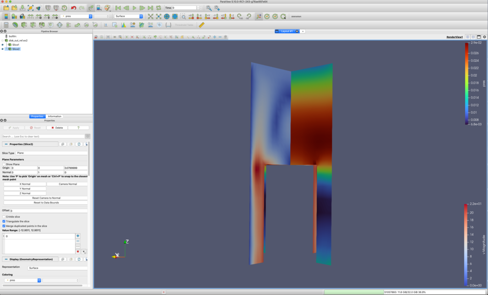
Slices

• File → Open → Examples → disk_out_ref.exo.. On the Properties tab, click Apply.
• +X
• Filters → Common → Slice. Apply. Unselect the Show Plane.
• Color by: v.
• In the pipeline browser, select disk_out_ref.exo
• Filters → Common → Slice. Y Normal. Apply. Unselect the Show Plane.
• Color by: pres.
• View → Color Map Editor → Presets (the little envelope with a heart) → Turbo.
• With the mouse, rotate the slices around so you can see both surfaces.

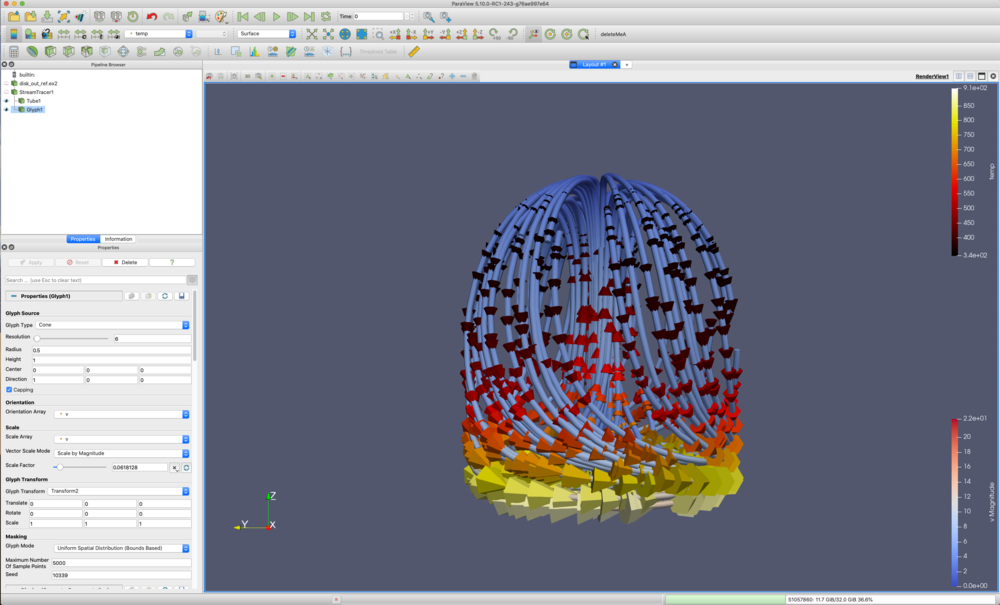
Stream Tracers - lines and tubes

• File → Open → Examples → disk_out_ref.exo.. On the Properties tab, click Apply.
• +X
• Filters → Common → Stream Tracer. v. Seed Type: Point Cloud. Uncheck Show Sphere. Apply.
• Color by: v.

Lines don't color as nicely as surfaces. Lets add a tube filter around each streamline.

• Filters → Search. Type Tube. Apply.

Now, we want to know which directions the particles are moving. We will use a glyph filter. Note we place the glyph filter on the streamline, not the tube.

• Select StreamTracer in the Pipeline Browser.
• Filters → Common → Glyph. Glyph Type: Cone. Orientation Array: v. Scale Array: v . Very Important - Scale Factor select the recycle button to the right. Apply.
• Color by: temp.
• View → Color Map Editor → Presets (the little envelope with a heart) → Black Body Radiation.
• Reset

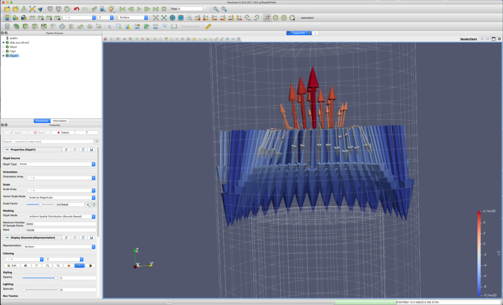
Glyphs perpendicular to a slice

• File → Open → Examples → disk_out_ref.exo.. On the Properties tab, click Apply.
• +X

Lets create a half slice. This will be used as the seed plane for glyphs.

• Filters → Common → Slice. Origin 0, 0, 5. Uncheck Show Plane. Apply.
• Filters → Common → Clip. Uncheck Show Plane. Apply.

Now, apply glyphs.

• Filters → Common → Glyph. Glyph Type: Arrow. Orientation Array: v. Scale Array: v . Very Important - Scale Factor select the recycle button to the right. .5X. .5X. Apply.
• Color by: v. Change Magnitude to Z.

Let's put these glyphs back into context by showing the original dataset.

• Select disk_out_ref.exo in the Pipeline Browser. Representation: wireframe. On the Properties tab, change Opacity to 0.3.
• Use the mouse to zoom into the glyph vectors.

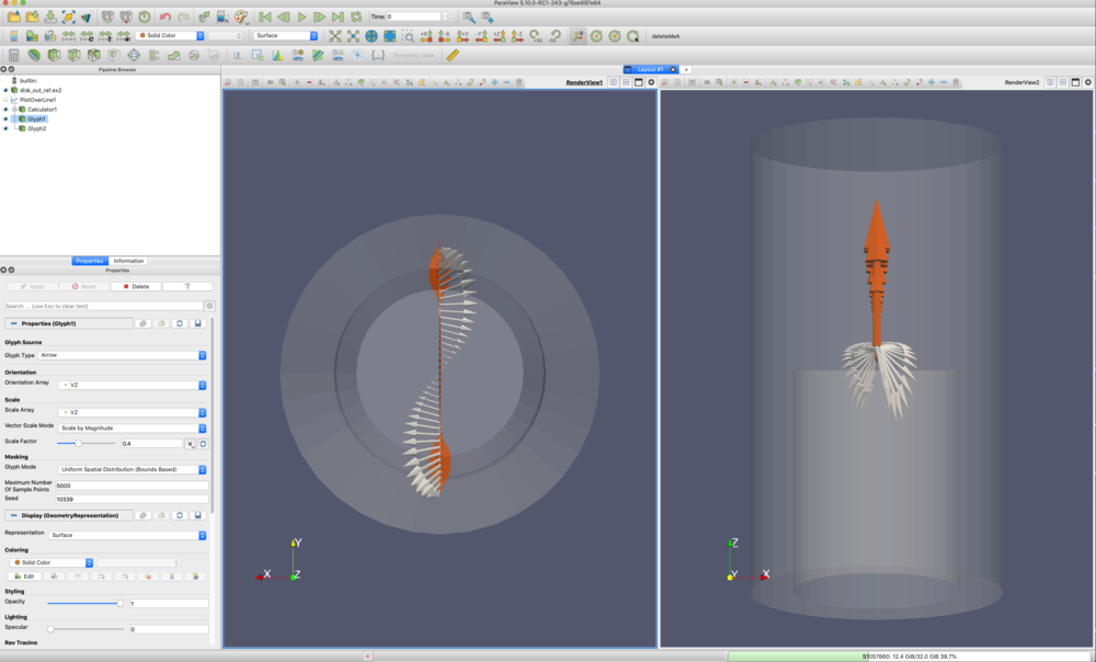
Flow in a fluid

To show a velocity profile we need to sample the dataset with a line, and then create glyphs off of this line. This can be done using a trick in ParaView, i.e., the Plot over Line filter. Note that a Resample to Line filter will be added in ParaView 5.11 or so.

• File → Open → Examples → disk_out_ref.exo.. On the Properties tab, click Apply.

Lets sample over a line.

• Filters → Data Analysis → Plot over Line. Y Axis. Change the Z component of the line to 1. Change the Resolution to 40. Apply.
• Close the LineChartView.
• In the Pipeline Browser, turn visibility off for disk_out_ref.exo.

We now have a line sampled through the fluid. Lets calculate the negative Z component of V (so it goes the opposite direction on the line from V). That way we can have two profiles, one with V, and one with Vz.

• Filters → Common → Calculator. Change Result to Vz. Use 0*iHat+0+jHat+-v_Z*kHat for the formula. Apply.

Now we want to create two Glyphs - one from the Calculator filter, and one directly from the Plot over Line filter.

• The Calculator filter should still be highlighted in the Pipeline Browser.
• Filters → Common → Glyph. Glyph Type: Arrow. Orientation Array: Vz. Scale Array: Vz . Very Important - Scale Factor select the recycle button to the right. .5X. .5X. Apply.
• Click on the Color Editor icon. Change the color to Orange. Apply.
• In the Pipeline Browser select the Plot over Line filter.
• Filters → Common → Glyph. Glyph Type: Arrow. Orientation Array: v. Scale Array: v . Very Important - Scale Factor select the recycle button to the right. Apply.

Let's put these glyphs back into context by showing the original dataset.

• Select disk_out_ref.exo in the Pipeline Browser. On the Properties tab, change Opacity to 0.3.

Just to create a nice image, I'm going to split the views horizontally, and show this visualization also from the side.